Big Picture

Because neural network comes with lots of mathematical notations (e.g. linear algebra, partial derivative sign , summation sigma notation and fractions), and many alphabets (meaning you are free to choose whatever you want), I think it's easy to get lost. So I describe the big picture of neural network as followed. For now, we don't care about what it means so much because we will go in detail later.

1. Initialize parameters (weights and biases)
2. Repeat the following until the loss becomes small
  i. With current parameters, compute predicted Y
  ii. Compute cost between actual Y and predicted Y
  iii. Compute the derivative of the cost with respect to parameters
  iv. Update current parameters by gradient descent
3. Predict by forward propagation with the updated parameters

People say the above i. step the forward propagation, and the iii. step the backward propagation. So I think we can simplify the above as followed.

Repeat this
1. Forward propagation
2. Compute cost
3. Backward propagation
4. Gradient descent

I oversimplied it because I wanted to emphasize that's the essence of the neural network, before we go to the details.

Forward Propagation

People use two type of parameters, called weight and called bias. for the linearly computed result. as the output of activation function. Activation function is a function which, given the input of linear combination, converts it to nonlinear output. We add this function because we want the model to capture a non-linear complex data relationship. In math,

represents any activation function and you are free to choose. So a linear function is okay too, but as described, people use a non-linear function. Also there are the non-linear functions that people tend to choose. These are sigmoid (), hyperbolic tangent (tanh) and rectified linear unit (ReLU). We see how those functions behave below.

import math

def sigmoid(x):
    return 1 / (1 + math.exp(-x))

def tanh(x):
    return (math.exp(x) - math.exp(-x)) / (math.exp(x) + math.exp(-x))

def relu(x):
    return max(0, x)

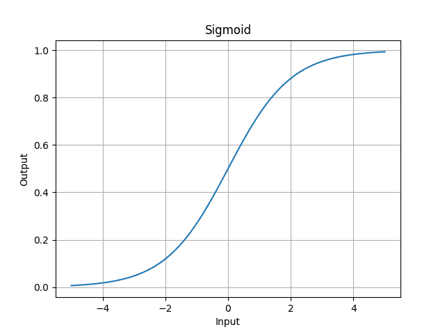
• sigmoid is something we want the output to be between 0 and 1.
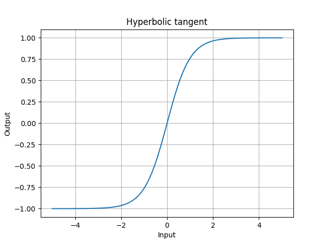
• tanh is between -1 and 1
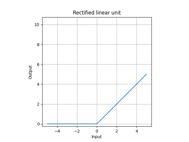
• relu is if input is positive, do nothing, but if negative, all 0.

In math, sigmoid is,

Tanh is,

ReLU is,

why we need to use non-linear activation. We see why by stacking 2 linear functions. Because we don't use non-linear activation and in practice it means don't use activation function at all to have linear activation, .

By substituting the first equation to the second,

Let be and be .

This is a linear equation. So composition of linear functions is a linear function. If the data has a non-linearity, the neural network which only uses linear activations cannot express the relationship.

We go back to the previous linear equation and non-linear equation. In neural network, we are allowed to repeat it as many as we want. We can stack them many times. We can have as many layers as we want. Use . is th layer in a neural network with layers in total.

For example, the input layer is,

The output layer is,

Notice that when we have layers in total, is our neural network model output. In the real-world problem, we are required to make regression or binary classification. So in the of the final layer, the choice of the activation function depends on our problem.

• If we need to make binary classification, needs to be a sigmoid function.
• If we are asked to make regression, is not a non-linear function. Just use the itself, because it will be a real number output computed by linear combination.

When a neural network has no hidden layers and one unit in output layer, meaning we are not repeating or stacking layers in neural network,

• If output layer is linear activation, it's linear regression because , same as
• If output layer is sigmoid activation, it's logistic regression because where , same as

We check the dimension of weights and biases . is the number of units (or nodes) in layer . Use for the units of input layer, so is equal to the number of features . is the number of example (or data).

Bias is always one column, so to make the following calculation possible, broadcasting happens to bias in programming computation. For example, is the number of examples (or data).

In linear algebra, you cannot do element-wise addtion between and . So the bias column is applied to each column in . It is broadcasting. To understand broadcasting, for example, if we have and and ,

Notice that and are repeated in each column.

Compute Cost

We define cost as the average of the loss from the individual examples like below. is the number of example (data).

We have and at the left side, because our prediction is computed by using parameters and , so the cost depend on what numbers we use in parameters. is a loss function. It's not using an explicit loss function, so we are free to choose it. For example, squared error loss , absolute loss . If our problem is binary classification, we can use the loss function in logistic regression of , called cross-entropy loss.

We will come back to the average part in backward propagation.

Our goal is to minimize this cost function. In math,

It means that we want to minimize the cost function using an optimal set of parameters and .

Backward Propagation

In forward propagation, we sequentially computed from input layer with the given data to output layer for our prediction . Contast to that, in backward propagation, we start from the output layer to input layer. The goal of the backward propagation is to compute gradient of the cost function with respect to parameters and for the following process of gradient descent. and exist in each layer in neural network. We will see that, to compute each derivative, each layer requires the derivative from the previous layers.

The reason why we have a sequence of derivative fractions is becuase is the cost of , , and

Backward propagation requires the derivative of the activation functions .

Derivative of sigmoid is,

Derivative of hyperbolic tangent (tanh) is,

Derivative of rectified linear unit (ReLU) is,

Gradient Descent

is a learning rate.

Math behind Neural Network Binary Classification

I think the backward propagation part doesn't look clear unless we have a concrete neural network architecture. Here, we use ReLU for all the activation functions in the hidden layers, and use sigmoid for the output layer.

So this neural network does a binary classification. So the neural network architecture is,

Linear () → Relu activation → Linear () → Relu → ... → Linear() → Sigmoid activation

We skip the forward propagation part because it's only about doing linear combination of and put to the ReLU activation function.

In backward propagation, we start from the gradient in the output layer. is the number of examples. is a single actual response. is a single predicted response. It uses the following cost function, called cross-entropy cost, because of binary classification. because is the output of the sigmoid activation at the output layer. The cost function is,

In backward propagation, the first derivative we need to compute is,

To make clear what's happening, instead of the cost of the entire examples, we look at a single .

Derivative of loss function with respect to is, by derivative of log and chain rule,

So we have,

So we found that we just element-wise apply to and for

What we need to compute next in backward propagation is,

To make things clear, we go back again to a single example case. notice that because we are doing binary classification and the output layer is sigmoid activation. We have,

By using the previously found result,

So we found that is just element-wise

Finally we can go to and , because we want these derivatives to do gradient descent to update parameters and . We needed and for this purpose.

By going back to a single example again, we have . It's easy to see,

By previously found result in the chain, the derivative of the loss with respect to weight is,

The derivative of the loss with respect to bias

In the entire data,

We have because we defined the cost function is the average of the loss of the individual examples. So the derivative of cost function with respect to will be,

We don't forget the gradient descent to update and

For the next previous layer in backward propagation, we need to find . In a single example, we have

So the derivative with respect to is,

The derivative of the loss with respect to is,

Element-wise apply the above to .

To continue the other layers in backward propagation, computation for the derivative with respect to will be different because the hidden layers use Relu activation. But it will be simpler, because the derivative of Relu is 1 if positive and 0 if negative. Keep repeating the above processes up to the input layer. For this, I replace the math with code in the following.

import numpy as np


def relu(Z):
    A = np.maximum(0, Z)
    cache = Z
    return A, cache


def relu_backward(dA, cache):
    Z = cache
    dZ = np.array(dA, copy=True)
    dZ[Z <= 0] = 0
    return dZ


def sigmoid(Z):
    A = 1 / (1 + np.exp(-Z))
    cache = Z
    return A, cache


def sigmoid_backward(dA, cache):
    Z = cache
    s = 1 / (1 + np.exp(-Z))
    dZ = dA * s * (1 - s)
    return dZ


def initialize_parameters(layer_dims, seed):
    """
    Argument:
    layer_dims: List of integers representing dimenstions of each layer
    Return:
    parameters: Dictionary containing weight matrices for W (n_l, n_{l - 1}) and bias columns (n_l, 1)
    """
    np.random.seed(seed)
    parameters = {}
    L = len(layer_dims)
    # Start from 1 to avoid index out of bound
    for l in range(1, L):
        # Initialize weights with small numbers so multiply by 0.01
        parameters[f'W{l}'] = 0.01 * np.random.randn(layer_dims[l], layer_dims[l - 1])
        # Initialize bias with zero
        parameters[f'b{l}'] = np.zeros((layer_dims[l], 1))
    return parameters


def linear_forward(A, W, b):
    Z = np.dot(W, A) + b
    cache = (A, W, b)
    return Z, cache


def linear_activation_forward(A_prev, W, b, activation):
    Z, linear_cache = linear_forward(A_prev, W, b)

    if activation == 'relu':
        A, activation_cache = relu(Z)
    elif activation == 'sigmoid':
        A, activation_cache = sigmoid(Z)
        
    cache = (linear_cache, activation_cache)
    
    return A, cache


def forward_propagation(X, parameters):
    caches = []
    # A^0 = X
    A = X
    # // 2 because parameters are doubled by w and b
    L = len(parameters) // 2
    
    # Hidden layers
    for l in range(1, L):
        A, cache = linear_activation_forward(
            A,
            parameters[f'W{l}'],
            parameters[f'b{l}'],
            # All the hidden layers use ReLU in this example
            activation='relu'
        )
        caches.append(cache)
        
    # Output layer
    # AL = sigmoid(W^L A^{L - 1} + b^L) = \hat{Y}
    AL, cache = linear_activation_forward(
        A,
        parameters[f'W{L}'],
        parameters[f'b{L}'],
        # Use sigmoid activation because this example is binary classification
        activation='sigmoid'
    )
    caches.append(cache)
    
    return AL, caches


def compute_cost(AL, Y):
    """
    Argument:
    AL: Output of sigmoid activation, so equal to \hat{y}
    Y: (1, number of examples)
    """
    m = Y.shape[1]
    # Compute cross-entropy cost
    # np.multiply is element-wise multiplication
    cost = (-1 / m) * np.sum(np.multiply(Y, np.log(AL)) + np.multiply(1 - Y, np.log(1 - AL)))
    # np.squeeze removes all the length 1 dimensions, so [[1]] goes to 1, shape is ()
    cost = np.squeeze(cost)
    return cost


def linear_backward(dZ, cache):
    A_prev, W, b = cache
    m = A_prev.shape[1]
    dW = (1 / m) * np.dot(dZ, A_prev.T)
    db = (1 / m) * np.sum(dZ, axis=1, keepdims=True)
    dA_prev = np.dot(W.T, dZ)
    return dA_prev, dW, db


def linear_activation_backward(dA, cache, activation):
    linear_cache, activation_cache = cache
    
    if activation == 'relu':
        dZ = relu_backward(dA, activation_cache)
    elif activation == 'sigmoid':
        dZ = sigmoid_backward(dA, activation_cache)
    
    dA_prev, dW, db = linear_backward(dZ, linear_cache)
    
    return dA_prev, dW, db


def backward_propagation(AL, Y, caches):
    # Gradients
    grads = {}
    L = len(caches)
    m = AL.shape[1]
    # Make AL have the same shape as AL (Y hat)
    Y = Y.reshape(AL.shape)
    
    # Derivative of cost function with respect to A (sigmoid activation at the output layer)
    dAL = - (np.divide(Y, AL) - np.divide(1 - Y, 1 - AL))
    
    current_cache = caches[-1]
    grads[f'dA{L - 1}'], grads[f'dW{L}'], grads[f'db{L}'] = linear_activation_backward(
        dAL,
        current_cache,
        'sigmoid'
    )
    
    # e.g. for i in reversed(range(3)): (2, 1, 0), 
    # So it's (0, 1, 2) and then reverse it
    for l in reversed(range(L - 1)):
        current_cache = caches[l]
        grads[f'dA{l}'], grads[f'dW{l + 1}'], grads[f'db{l + 1}'] = linear_activation_backward(
            grads[f'dA{l + 1}'],
            current_cache,
            'relu'
        )
    
    return grads


def update_parameters(parameters, grads, learning_rate):
    # // 2 because parameters are doubled by w and b
    L = len(parameters) // 2
    
    for l in range(L):
        # Gradient descent
        parameters[f'W{l + 1}'] = parameters[f'W{l + 1}'] - learning_rate * grads[f'dW{l + 1}']
        parameters[f'b{l + 1}'] = parameters[f'b{l + 1}'] - learning_rate * grads[f'db{l + 1}']
        
    return parameters


# For training
# When input has 100 features, and to make 4 layers neural network
# Last element needs to be 1 because of binary classification
layer_dims = [100, 20, 7, 5, 1]
learning_rate = 0.001
num_iterations = 1000
np.random.seed(0)

# X: (p by n)
X = np.array([])
# Y: (1 by n)
Y = np.array([])

# Initialize parameters
parameters = initialize_parameters(layer_dims)

# Store cost computed from each iteration
costs = []

# Keep training until num_iterations times
for _ in range(num_iterations):
    
    # Forward propagation to compute Y hat
    AL, caches = forward_propagation(X, parameters)
    
    # Compute cost
    cost = compute_cost(AL, Y)
    
    # Backward propagation to compute gradients
    grads = backward_propagation(AL, Y, caches)
    
    # Update parameters by gradient descent
    parameters = update_parameters(parameters, grads, learning_rate)
    
    # Save cost
    costs.append(cost)

# Visualize cost reduced over training iterations
plt.plot(np.squeeze(costs))
plt.ylabel('cost')
plt.xlabel('iterations')
plt.title("Learning rate =" + str(learning_rate))
plt.show()

# For predicting
def predict(X, y, parameters):
    m = X.shape[1]
    n = len(parameters) // 2
    p = np.zeros((1, m))
    
    # Forward propagation to compute Y hat
    # In prediction, we don't need caches
    probas, _ = forward_propagation(X, parameters)
    
    # Convert the predicted probability to binary prediction
    for i in range(probas.shape[1]):
        if probas[0,i] > 0.5:
            p[0,i] = 1
        else:
            p[0,i] = 0
            
    print(f'Accuracy: {np.sum((p == y) / m)}')
    
    return p